How to diagnose fuel properties in WRF-SFIRE
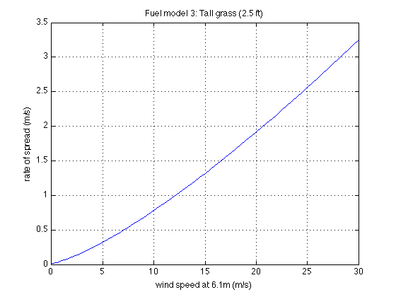
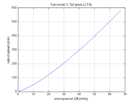
The fuel properties in WRF-Fire are given in file namelist.fire. These serve to create coefficients in the Rothermel's formula. To aid diagnostics it is useful to graph the resulting fire spread rate as a function of wind and slope. The graphs are available in metric units, as well as in English units for direct comparison with the published spread rate graphs for the Scott-Burgan fuel categories.
Prerequisites
Location of the codes
- The fuel properties of every category of the fuel are defined in file namelist.fire, which needs to be in the current directory.
- The fire rate of spread computation is done in file WRFV3/phys/module_fr_sfire_phys.F split between two subroutines. First, the coefficients at every point are precomputed from fuel properties in subroutine set_fire_params at initialization. In every time step, the spread rate at a point is then computed from those coefficients in subroutine fire_ros.
- The computation has been duplicated in Matlab for diagnostic purposes in file other/Matlab/vis3d/fire_ros.m
- The plot routine to create graphs like shown here is other/Matlab/vis3d/plot_fuel.m
Heat flux diagnostics
- plot_fuel also computes and prints several diagnostic quantities derived from fuel properties, including total heat density generated by the combustion of the fuel over time (J/m2), and the maximal heat flux density (W/m2) from the initial slope of the fuel loss curve. These can be compared with the statistic printed by WRF-Fire while running (maximal heat flux density, total heat flux of the fire, total heat generated by the fire) for validation.
Step-by-step instructions
- Run WRF-Fire, you can kill it right after the the first time step. There will be file fuels.m created in the current directory.
- Start Matlab in the directory test/em_fire to set up the search path properly.
- In Matlab, navigate to the directory with the fuels.m file
- Type fuels. This will create variable fuel. Say you want to check fuel 3. Type fuel(3) to see what is there.
- Type plot_fuel(fuel(3)) to create the graph below in metric units, and plot_fuel(fuel(3),'sb') for the same units as in Scott and Burgan (2005). Note: The graph data were created in WRF-Fire and stored in the fuel variable.
- Type edit fire_ros to see the fire spread rate calculation recreated in Matlab.
- Type big(check_ros(fuel)) to make sure the calculation in Matlab is the same as in WRF-Fire, it should return rounding error only (less than 1e-4)
Works with
- WRF-Fire branch fireflux 16 Sep 2010 and hopefully later
- Matlab R2010a and hopefully later
References
- Anderson, H. E., 1982. Aids to determining fuel models for estimating fire behavior. U.S. Forest Service General Technical Report INT-122. Ogden, UT. pdf (The original 13 fuel models)
- Baughman, R. G. and F. A. Albini.,1980. Estimating midflame windspeeds. In Sixth Conference on Fire and Forest Meteorology, Seattle, WA (Society of American Foresters) pdf (Windspeed reduction from 20ft)
- Rothermel, R.C., 1972. A mathematical model for predicting fire spread in wildland fuels. Res. Pap. INT-115. Ogden, UT: U.S. Department of Agriculture, Forest Service, Intermountain Forest and Range Experiment Station. 40 pp. pdf (The original for reference)
- Rothermel, R. C., 1983. How to predict the spread and intensity of forest and range fires. U.S. Forest Service General Technical Report INT-143. Ogden, UT. pdf (Updated version)
- Scott, J. H. and Burgan, R. E., 2005. Standard fire behavior fuel models: a comprehensive set for use with Rothermel's surface fire spread model. Gen. Tech. Rep. RMRS-GTR-153. Fort Collins, CO: U.S. Department of Agriculture, Forest Service, Rocky Mountain Research Station, 72 pp. pdf (More detailed fuel models, with rate of spread curves)

