How to run WRF-Fire with real data
- This is an archived historical WRF-Fire/WRF-SFIRE page. Please go to Running WRF-SFIRE with real data in the WRFx system for the current software version.
Running WRF-Fire with real data is a process very similar to running WRF with real data for weather simulations. The WRF users page has many documents and tutorials outlining this process. The purpose of this page is to provide a tutorial for using real data with WRF-Fire starting from scratch. We begin with a quick outline of the steps involved including links to the output of each step. The user can use these linked files to start from any step or to verify their own results. Due to platform and compiler differences your output might differ slightly from those provided.
This page refers to data sources for the USA only. For other countries, you will need to make appropriate modifications yourself.
Outline
- Obtain WRF-Fire source code.
- Compile target em_real.
- Compile WPS.
- Configure your domain.
- Download geogrid datasets.
- Converting fuel data.
- Run the geogrid executable.
- Download atmospheric data.
- Run the ungrib executable.
- Run the metgrid executable.
- Run real.exe and wrf.exe.
Compiling WPS
After you have compiled WRF, you then need to go into the subdirectory WPS and run
./configure. This will present you with a list of configuration options similar to those given by WRF.
You will need to chose one with the same compiler that you used to compile WRF. Generally, it is unnecessary to compile WPS with parallel support.
GRIB2 support is only necessary if your atmospheric data source requires it. Once you have chosen a configuration, you can compile with
./compile >& compile.log
Make sure to check for errors in the log file generated.
Configuring the domain
The physical domain is configured in the geogrid section of namelist.wps in the WPS directory. In this section, you should define the geographic projection with map_proj, truelat1, truelat2, and stand_lon. Available projections include 'lambert', 'polar', 'mercator', and 'lat-lon'. The lower left corner of the domain is located at ref_lon longitude and ref_lat latitude. The computational grid is defined by e_we/e_sn, the number of (staggered) grid points in the west-east/south-north direction, and the grid resolution is defined by dx and dy in meters. We also specify a path to where we will put the static dataset that geogrid will read from, and we specify the highest resolution (30 arc minutes) that this data is released in.
&geogrid
 e_we              =  43,
 e_sn              =  43,
 geog_data_res     = '30s',
 dx = 60,
 dy = 60,
 map_proj  = 'lambert',
 ref_lat   =  39.70537,
 ref_lon   = -107.2907,
 truelat1  =  39.338,
 truelat2  =  39.338,
 stand_lon = -106.807,
 geog_data_path = '../../wrfdata/geog'
/
The share section of the WPS namelist defines the fire subgrid refinement in subgrid_ratio_x and subgrid_ratio_y. This means that the fire grid will be a 10 time refined grid at a resolution of 6 meters by 6 meters. The start_date and end_data parameters specify the time window that the simulation will be run in. Atmospheric data must be available at both temporal boundaries. The interval_seconds parameter tells WPS the number of seconds between each atmospheric dataset. For our example, we will be using the NARR dataset which is released daily every three hours or 10,800 seconds.
&share
 wrf_core = 'ARW',
 max_dom = 1,
 start_date = '2005-08-28_12:00:00',
 end_date   = '2005-08-28_15:00:00',
 interval_seconds = 10800,
 io_form_geogrid = 2,
 subgrid_ratio_x = 10,
 subgrid_ratio_y = 10,
/
The full namelist used can be found here.
Obtaining data for geogrid
First you must download and uncompress the standard geogrid input data. This is a 429 MB compressed tarball that uncompresses to around 11 GB. It contains all of the static data that geogrid needs for a standard weather simulation; however, for a WRF-Fire simulation we need to fill in two additional fields that are too big to release in a single download for the whole globe. We first need to determine the approximate latitude and longitude bounds for our domain.
We know the coordinates in the lower left corner from the ref_lon and ref_lat parameters of the namelist. We can estimate the coordinates of the upper right corner by the approximate ratio 9e-6 degrees per meter. So, the upper right corner of our domain is at approximately -107.2675 longitude and 39.7286 latitude. For the purposes of downloading data, we will expand this region to the range -107.35 through -107.2 longitude and 39.6 through 39.75 latitude.
Downloading fuel category data
For the United States, Anderson 13 fuel category data is available at the landfire website. Upon opening the national map,
click roughly on your are of interest, the map will zoom in, you will see a menu on the top of the screen. Click on the earth icon, that should display a drop down menu, and select option 'Download Data'

This will open a new window on the right. Click on 'x y' icon that will open a form that lets you key in the the longitude and latitude range of your selection. In this window, we will input the coordinates computed earlier, and below we will select 'LF_2014 (LF_140)', then 'Fuel', and 'us_140 13 Fire Behavior Fuel Models-Anderson, and click 'Add Area' button.

In the next window, click on "modify data request". This window lists all of the available data products for the selected region. You want to check the box
next to "US_140 13 Fire Behavior Fuel Models-Anderson" and change the data format from "ArcGRID_with_attribs" to "GeoTIFF_with _attribs". At the bottom make sure "Maximum size (MB) per piece:" is set to 250. Then go to the bottom of the page and click "Save Changes".

Finally, click "Download". The file will be a compressed archive containing, among others, a GeoTIFF file. The name of the file will be different for each request,
but in this example we have lf02588871.zip containing the GeoTIFF file lf02588871.tif, which can be found here, File:Lf02588871.tif.
Downloading high resolution elevation data
For the United States, elevation data is also available at the landfire website. Repeat the steps described above for downloading the fuel data, but instead of selecting "LF2014 (LF_140) US_140 13 Fire Behavior Models-Anderson, this time select: "Topographic" and "us Elevation".
 Again, we key in the coordinates determined before and click "Add Area".
In the next window click again "Modify Data Request", make sure only us_Elevation is selected, change format to "Geotiff" and click "Save Changes & Return to Summary"

In the next window you should be able to click "Download" in order to download the GeoTIFF file containing topography. This sample file can be downloaded from here:
File:09159064.tif
Converting fuel data
This section describes converting data from geotiff to geogrid format. Alternatively, you can use the version of geogrid from our repository and read the geotiff file directly. For details see WPS_with_GeoTIFF_support.
In order for geogrid to be able to read this data, we need to convert it into an intermediate format. We will be using a utility program released with autoWPS to accomplish this. For information on how to obtain and compile this tool, see How_to_convert_data_for_Geogrid_(archived). We will place the convert_geotiff.x binary and the GeoTIFF data files in the main WPS directory. To convert the fuel category data, we will create new directories inside the WPS directory called landfire_data and ned_data. Inside the landfire_data directory, we issue the following command to convert the fuel category data.
../convert_geotiff.x -c 13 -w 1 -u "fuel category" -d "Anderson 13 fire behavior categories" ../lf02588871.tif
The resulting index file created as follows.
projection = albers_nad83
truelat1 = 29.500000
truelat2 = 45.500000
stdlon = -96.000000
known_x = 1
known_y = 606
known_lat = 39.747818
known_lon = -107.373398
dx = 3.000000e+01
dy = 3.000000e+01
type = categorical
signed = yes
units = "fuel category"
description = "Anderson 13 fire behavior categories"
wordsize = 1
tile_x = 100
tile_y = 100
tile_z = 1
category_min = 1
category_max = 14
tile_bdr = 3
missing_value = 0.000000
scale_factor = 1.000000
row_order = bottom_top
endian = little
We have chosen to set the word size to 1 byte because it can represent 256 categories, plenty for this purpose. Notice that the program has changed the number of categories to 14 and uses the last category to indicate that the source data was out of the range 1-13. For the fuel category data, this represents that there is no fuel present, due to a lake, river, road, etc.
We can check that the projection information entered into the index file is correct, by running the listgeo binary that is installed with libGeoTIFF. In this case, listgeo tells us that the source file contains the following projection parameters.
Projection Method: CT_AlbersEqualArea
   ProjStdParallel1GeoKey: 29.500000 ( 29d30' 0.00"N)
   ProjStdParallel2GeoKey: 45.500000 ( 45d30' 0.00"N)
   ProjNatOriginLatGeoKey: 23.000000 ( 23d 0' 0.00"N)
   ProjNatOriginLongGeoKey: -96.000000 ( 96d 0' 0.00"W)
   ProjFalseEastingGeoKey: 0.000000 m
   ProjFalseNorthingGeoKey: 0.000000 m
GCS: 4269/NAD83
Datum: 6269/North American Datum 1983
Ellipsoid: 7019/GRS 1980 (6378137.00,6356752.31)
Prime Meridian: 8901/Greenwich (0.000000/  0d 0' 0.00"E)
Projection Linear Units: 9001/metre (1.000000m)

Corner Coordinates:
Upper Left    ( -963525.000, 1916445.000)  (-107.3734004,39.7478163)
Lower Left    ( -963525.000, 1898265.000)  (-107.3478974,39.5867431)
Upper Right   ( -948885.000, 1916445.000)  (-107.2021990,39.7632976)
Lower Right   ( -948885.000, 1898265.000)  (-107.1770727,39.6021889)
Center        ( -956205.000, 1907355.000)  (-107.2751374,39.6750401)
We can see that the conversion detected the projection correctly. The small difference in the coordinates of the upper left corner reported by listgeo and that in the index file is due to floating point error and is much less than the resolution of the data.
Finally, we go to the ned_data directory to convert the ZSF variable. In this case, we issue the following command.
../convert_geotiff.x -u meters -d 'National Elevation Dataset 1/3 arcsecond resolution' ../09159064.tif
This produces the following index file.
projection = regular_ll
known_x = 1
known_y = 1621
known_lat = 39.750092
known_lon = -107.350090
dx = 9.259259e-05
dy = 9.259259e-05
type = continuous
signed = yes
units = "meters"
description = "National Elevation Dataset 1/3 arcsecond resolution"
wordsize = 2
tile_x = 100
tile_y = 100
tile_z = 1
tile_bdr = 3
missing_value = 0.000000
scale_factor = 1.000000
row_order = bottom_top
endian = little
Here we have used the default word size of 2 bytes and a scale factor of 1.0, which can represent any elevation in the world with 1 meter accuracy, which is approximately the accuracy of the source data.
Again, we compare the projection parameters in the index file with that reported by listgeo and find that the conversion was correct.
      Keyed_Information:
      GTModelTypeGeoKey (Short,1): ModelTypeGeographic
      GTRasterTypeGeoKey (Short,1): RasterPixelIsArea
      GeographicTypeGeoKey (Short,1): GCS_NAD83
      GeogCitationGeoKey (Ascii,6): "NAD83"
      GeogAngularUnitsGeoKey (Short,1): Angular_Degree
      End_Of_Keys.
   End_Of_Geotiff.

GCS: 4269/NAD83
Datum: 6269/North American Datum 1983
Ellipsoid: 7019/GRS 1980 (6378137.00,6356752.31)
Prime Meridian: 8901/Greenwich (0.000000/  0d 0' 0.00"E)

Corner Coordinates:
Upper Left    (-107.3500926,39.7500926)
Lower Left    (-107.3500926,39.6000000)
Upper Right   (-107.2000000,39.7500926)
Lower Right   (-107.2000000,39.6000000)
Center        (-107.2750463,39.6750463)
Finally, the converted data can be found here, File:Landfire data.tgz, and here, File:Ned data.tgz.
Running geogrid
The geogrid binary will create a netcdf file called geo_em.d01.nc. This file will contain all of the static data necessary to run your simulation. Before we can run the binary, however, we must tell geogrid what data needs to be in these files, where it can find them, and what kind of preprocessing we wnat done. This information is contained in a run-time configuration file called GEOGRID.TBL, which is located in the geogrid subdirectory. The file that is released with WPS contains reasonable defaults for the variables defined on the atmospheric grid, but we need to add two additional sections for the two fire grid data sets that we have just created. We will append the following sections to the file geogrid/GEOGRID.TBL.
===============================
name=NFUEL_CAT
        priority=1
	dest_type=categorical
	dominant_only=NFUEL_CAT
	z_dim_name=fuel_cat
	halt_on_missing=yes
	interp_option=default:nearest_neighbor
	abs_path=./landfire_data
	subgrid=yes
==============================
name=ZSF
        priority = 1
        dest_type = continuous
        df_dx=DZDXF
        df_dy=DZDYF
        smooth_option = smth-desmth_special; smooth_passes=1
	halt_on_missing=yes
        interp_option = default:average_gcell(4.0)+four_pt+average_4pt
	abs_path=./ned_data
	subgrid=yes
==============================
For NFUEL_CAT, we will use simple nearest neighbor interpolation, while for ZSF, we will use bilinear interpolation with smoothing. Other configurations are possible. See the WPS users guide for further information. The full table used can be found here.
Once we make these changes to the GEOGRID.TBL file, and ensure that all of the directories are in the correct place (including the default geogrid dataset at ../../wrfdata), we can execute the geogrid binary.
./geogrid.exe
This will create a file called geo_em.d01.nc in the current directory, which can be found here, File:Geo em.d01.nc.gz. The contents of this file can be viewed using your favorite NetCDF viewer.
- geo_em.d01.nc
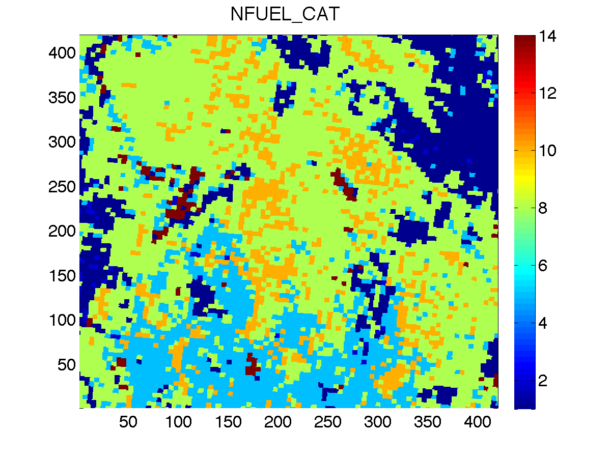
The fuel category data interpolated to the model grid.The
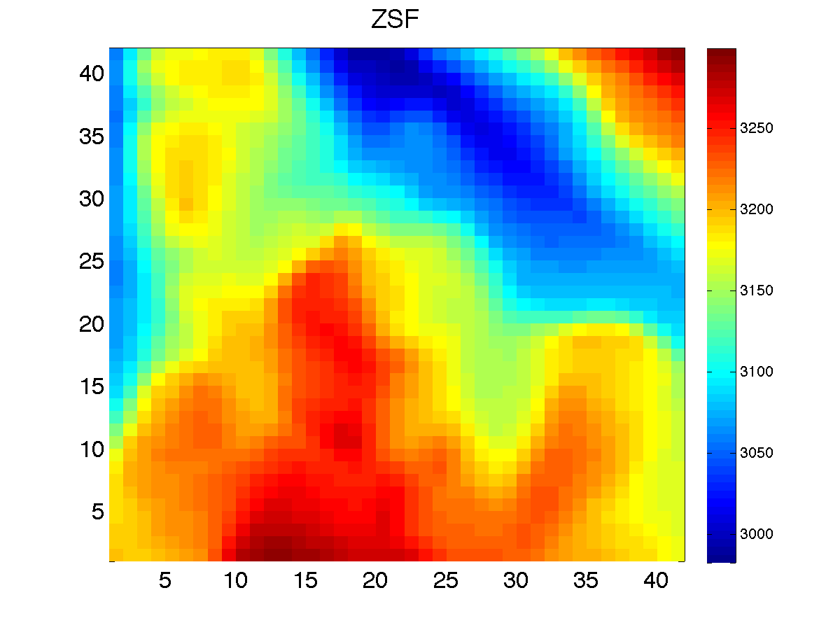
The high resolution elevation (1/3") data interpolated to the model grid.
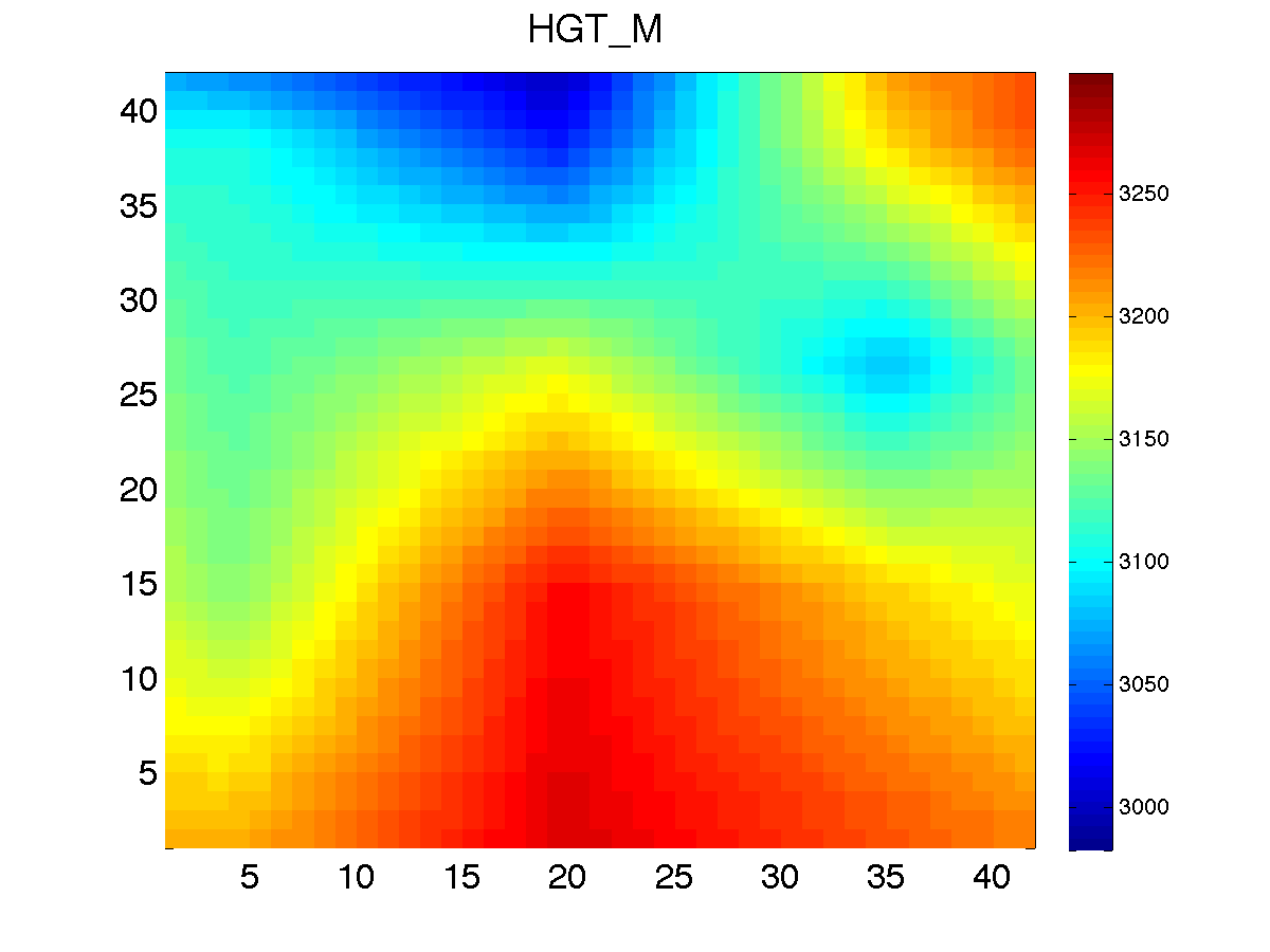
The low resolution elevation data (30") data interpolated to the atmospheric grid


Here, we have visualized the fire grid variables, NFUEL_CAT and ZSF, as well as the variable HGT_M, which is the elevation data used by the atmospheric model. We can compare ZSF and HGT_M to verify that our data conversion process worked. The colormaps of these two pictures have been aligned, so that we can make a quick visual check. As we see, the two images do have a similar structure and magnitude, but they do seem to suffer some misalignment. Given that the data came from two different sources, in two different projections, the error is relatively minor. Because WPS converts between projections in single precision, by default, there is likely a significant issue with floating point error. We may, in the future, consider making some changes so that this conversion is done in double precision.
Obtaining atmospheric data
There are a number of datasets available to initialize a WRF real run. The WRF users page lists a few. One challenge in running a fire simulation is finding a dataset of sufficient resolution. One (relatively) high resolution data source is the North American Regional Reanalysis (NARR). This is still only 32km resolution, so no small scale weather patterns will appear in our simulation. In general, we will want to run a series of nested domains in order to catch some small scale weather features; however, we will proceed with a single domain example.
The NARR datasets are available after 3 months at the following website, http://nomads.ncdc.noaa.gov/data/narr/. We will browse to the directory containing the data for August 28, 2005. Our simulation runs from the hours 12-15 on this day, so we will download the grib files for hours 12 and 15. You can get these files also from here, File:Narr-a 221 20050828 12-15.tgz.
Running ungrib
With the grib files downloaded, we need to link them into the WPS directory using the script link_grib.csh. This script takes as arguments all of the grib files that are needed for the simulation. In this case, we can run the following command in the WPS directory.
./link_grib.csh <path to>/*.grb
Substitute <path to> with the directory in which you have saved the grib files. This command creates a series of symbolic links with a predetermined naming sequence to all of the grib files you pass as arguments. You should now have two new soft links named GRIBFILE.AAA and GRIBFILE.AAB.
With the proper links in place, we need to tell ungrib what they contain. This is done by copying a variable table into the main WPS directory. Several variable tables are distributed with WPS which describe common datasets. You can find these in the directory WPS/ungrib/Variable_Tables. In particular, the file which corresponds to the NARR grib files is called Vtable.NARR, so we issue the following command to copy it into the current directory.
cp ungrib/Variable_Tables/Vtable.NARR Vtable
We are now ready to run the ungrib executable.
./ungrib.exe
This will create two files in the current directory named FILE:2005-08-28_12 and FILE:2005-08-28_15. You can download these files here, File:Ungrib output.tgz.
Running metgrid
Metgrid will take the files created by ungrib and geogrid and combine them into a set of files. At this point, all we need to do is run it.
./metgrid.exe
This creates two files named met_em.d01.2005-08-28_12:00:00.nc and met_em.d01.2005-08-28_15:00:00.nc, which you can download here, File:Metgrid output.tgz.
Running wrf
We are now finished with all steps involving WPS. All we need to do is copy over the metgrid output files over to our WRF real run directory at WRFV3/test/em_real and configure our WRF namelist. We will need to be sure that the domain description in namelist.input matches that of the namelist.wps we created previously, otherwise WRF will refuse to run. Pay particular attention to the start/stop times and the grid sizes. The fire ignition parameters are configured in the same way as for the ideal case. Relevant portion of the namelist we will use are given below.
 &time_control
 run_days                            = 0,
 run_hours                           = 0,
 run_minutes                         = 2,
 run_seconds                         = 0,
 start_year                          = 2005,
 start_month                         = 08,
 start_day                           = 28,
 start_hour                          = 12,
 start_minute                        = 00,
 start_second                        = 00,
 end_year                            = 2005,
 end_month                           = 08,
 end_day                             = 28,
 end_hour                            = 15,
 end_minute                          = 00,
 end_second                          = 00,
 interval_seconds                    = 10800
 input_from_file                     = .true.,
 history_interval_s                  = 30,
 frames_per_outfile                  = 1000,
 restart                             = .false.,
 restart_interval                    = 1,
 io_form_history                     = 2
 io_form_restart                     = 2
 io_form_input                       = 2
 io_form_boundary                    = 2
 /

 &domains
 time_step                           = 0,
 time_step_fract_num                 = 5,
 time_step_fract_den                 = 10,
 max_dom                             = 1,
 s_we                                = 1,
 e_we                                = 43,
 s_sn                                = 1,
 e_sn                                = 43,
 s_vert                              = 1,
 e_vert                              = 41,
 num_metgrid_levels                  = 30
 dx                                  = 60,
 dy                                  = 60,
 grid_id                             = 1,
 parent_id                           = 0,
 i_parent_start                      = 0,
 j_parent_start                      = 0,
 parent_grid_ratio                   = 1,
 parent_time_step_ratio              = 1,
 feedback                            = 1,
 smooth_option                       = 0
 sr_x                                = 10,
 sr_y                                = 10,
 sfcp_to_sfcp                        = .true.,
 p_top_requested                     = 10000
 /

 &bdy_control
 spec_bdy_width                      = 5,
 spec_zone                           = 1,
 relax_zone                          = 4,
 specified                           = .true.,
 periodic_x                          = .false.,
 symmetric_xs                        = .false.,
 symmetric_xe                        = .false.,
 open_xs                             = .false.,
 open_xe                             = .false.,
 periodic_y                          = .false.,
 symmetric_ys                        = .false.,
 symmetric_ye                        = .false.,
 open_ys                             = .false.,
 open_ye                             = .false.,
 nested                              = .false.,
 /
The full namelist used can be found here.
Once the namelist is properly configured we run the WRF real preprocessor.
./real.exe
This creates the initial and boundary files for the WRF simulation and fills all missing fields from the grib data with reasonable defaults. The files that it produces are wrfbdy_d01 and wrfinput_d01, which can be downloaded here File:Wrf real output.tgz.
Finally, we run the simulation.
./wrf.exe
The history file for this example can be downloaded here, File:Wrf real history.tgz.