How to interpret WRF variables
- Back to the WRF-SFIRE user guide.
This page describes the interpretation of selected atmospheric variables, which are important for fire visualization. See WRF documentation for further details.
Grid
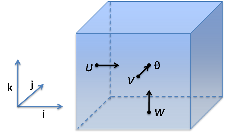
Grids in WRF are logically rectilinear. Variables for WRF cell indexed (i,j,k) can be located at one of 4 possible points. You can tell where by looking at the WRF registry or the attributes of NetCDF files, which WRF uses as I/O format. You can also tell by the fact that staggered variables have the staggered dimension larger by one, since there needs to be variable at the last boundary face.
- at the center of the cell - theta points, not staggered
- at the center of the left face - U point, staggered in X
- at the center of the front face - V point, staggered in Y
- at the center of the bottom face - W point, staggered in Z
Scalar variables (such as thermodynamical variables, hence the theta: temperature, pressure,...) generally live at theta-points. One exception is the geopotential, which lives at W-points. The documentation, some variable names, and comments in the WRF code also associate theta with the vertical position of the mid-plane of the cell and at W with the vertical position of the bottom of the cell.
The orientation of the axes in the real world, such as "east-west", in the order of increasing index, such as i, are defined in the registry. For postprocessing, they can be found at runtime as attributes in the NetCDF files.
Arrays
Arrays are stored in files and in memory. All arrays are described in the Registry, which is a collection of text files in WRFV3/Registry. The variable names in memory and in files are sometimes different.
Files are (by default) in NetCDF format. The values associated with the cell (i,j,k) at time step n are stored in the files as the array entry u(i,j,k,n), e.t.c. The value of the time at the step n is stored in character array Times(:,n).
While arrays in files are indexed as (i,j,k,n), arrays in memory are indexed as (i,k,j) by WRF coding conventions. Of course, there is no 4th index for the time step in arrays in memory, and in some arrays there is no vertical k dimension.
Wind
Components of the wind velocity vector U, V, W live at the corresponding points, hence the point names. These are in the geometrically horizontal and vertical directions. On flat ground, W on the first level k=1 is zero. However, when the ground has nonzero slope, the vertical velocity components W is generally not zero, because the normal vector to the ground is not vertical.
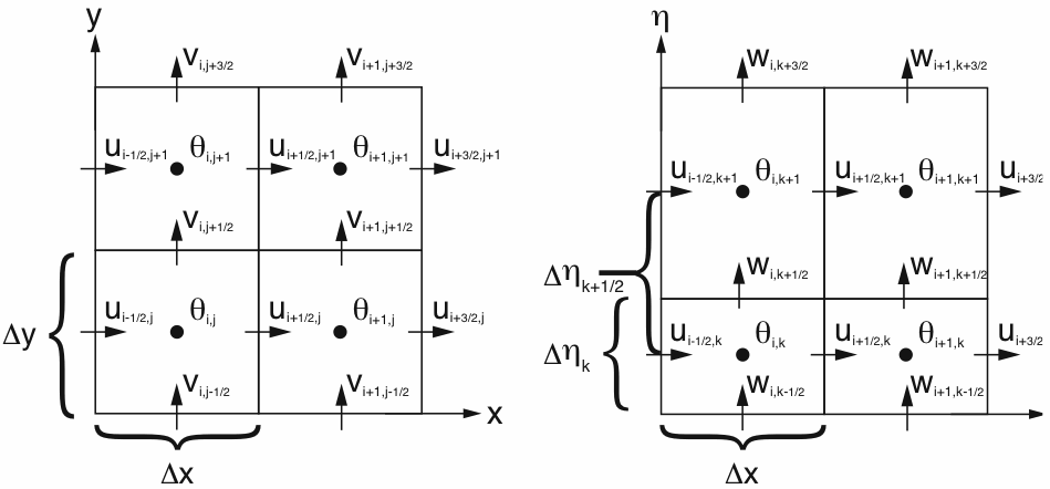
Note that the picture above center and right (from WRF documentation) use half integer indexing.
- The horizontal wind component Ui-1/2,j,k in the X direction is stored in the array entry u(i,j,k)
- The horizontal wind component Vi,j-1/2,k in the Y is stored in the array entry v(i,j,k)
- The vertical wind component Wi,j,k-1/2 is stored in the array entry w(i,j,k)
In particular, the lowest layer in WRF is k=1, and, on flat ground, w(:,:,1)=0, since the ground is impermeable in the normal direction. On a ground with nonzero slope, w(:,:,1)=0 is generally nonzero. The winds at the middle of the first layer, at the height eta1, are u(:,:,1), v(:,:,1), and they are generally nonzero.
Because the components of the wind velocity vector are on different staggered grids, and visualization software usually expects all three components of the velocity vector based at the same point, they need to be interpolated to theta-points (cell centers) for display:
- U_THETA(i,j,k) = 0.5*(U(i,j,k) + U(i+1,j,k))
- V_THETA(i,j,k) = 0.5*(V(i,j,k) + V(i,j+1,k))
- W_THETA(i,j,k) = 0.5*(W(i,j,k) + W(i,j,k+1))
Location
The longitude and latitude of the theta and U nodes are given by arrays XLONG and XLAT, which are set at initialization and then do not change. However the elevation has to be computed from the flow solution as geopotential height by
- ELEVATION_W(i,j,k) = (PHB(i,j,k) + PH(i,j,k))/9.81
where PHB + PH is the geopotential. PHB is constant, set at initialization, and PH, called perturbation geopotential, starts as zero and varies with time.
PH and PHB live at the W-points, thus the geopotential height at the lowest level is the same as terrain height
- ELEVATION_W(i,j) = PHB(i,j,1)/9.81
up to rounding error. This variable is also part of WRF state as z_at_w and its output to wrfout or wrfrst files can be enabled in the registry.
To find the elevation of the cell theta-points (the cell midplane, where the pressure and other variables than wind live), you need to interpolate between the elevation of the top and the bottom:
- ELEVATION_THETA(i,j,k) =0.5*(PHB(i,j,k) + PH(i,j,k) + PHB(i,j,k+1) + PH(i,j,k+1))/9.81
This variable is also part of WRF state as Z and its output to wrfout or wrfrst files can be enabled in the registry.
Temperature
Potential temperature in K is 300+T. The potential temperature is most suitable for visualization. However, the temperature as measured by instruments is sometimes needed for comparison. The potential temperature is converted by... coming soon
Pressure
coming soon
See also
- SFIRE variables
- WRF-Fire documentation
- WRF output fields from the WRF-ARW user's guide
- Grid: A Description of the Advanced Research WRF Version 3 (June 2008) Fig 7.3 page 59
- WRF Coding Conventions
- WRF Registry and Examples
- WRF v2 Software Tools and Documentation (there does not seem to be a document for V3?)
- Description of WRF Registry
- Moving from MM5 to WRF

